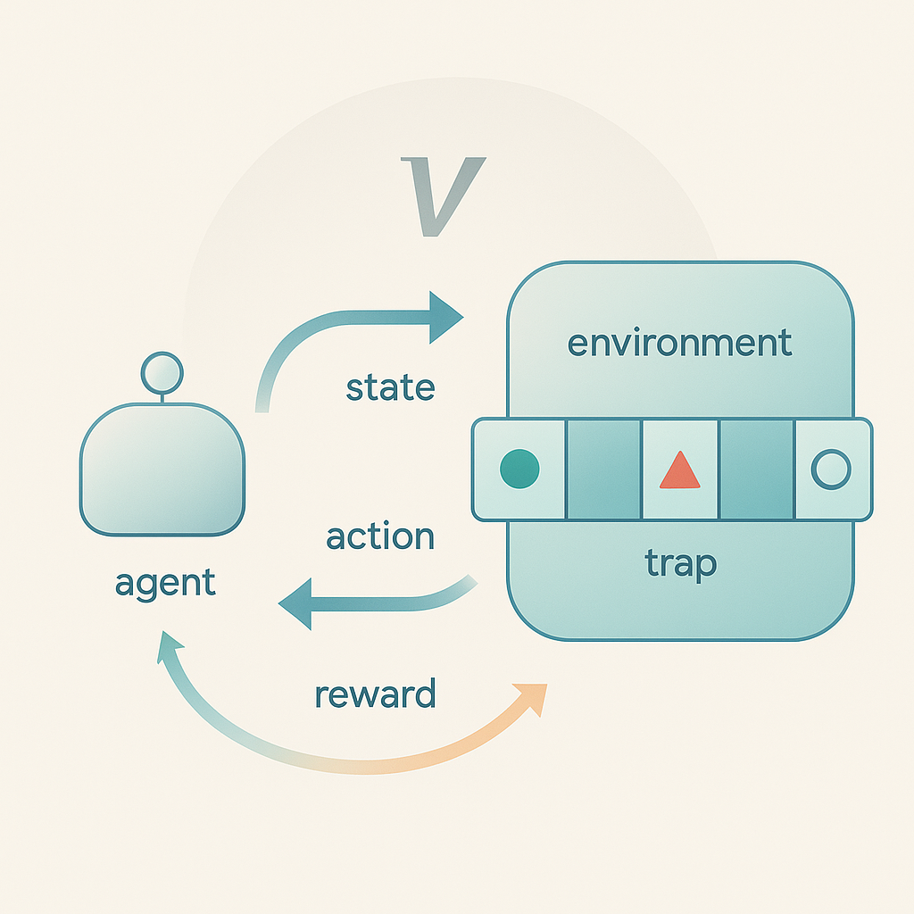
Reinforcement learning is neither supervised nor unsupervised – it learns from consequences. This article builds the vocabulary for the whole series: state, action, reward, policy, Markov property, discounting, Bellman equation. A runnable mini-env in pure numpy makes the concepts tangible.
1. The Problem: Learning Without a Teacher, but With Consequences
Classical supervised learning sees the correct label for every input. Unsupervised learning looks for structure without labels. Reinforcement learning gets no labels – only rewards, often long after the action.
"Reinforcement learning is learning what to do – how to map situations to actions – so as to maximize a numerical reward signal." – Sutton & Barto, Reinforcement Learning: An Introduction
The following table separates the three paradigms:
| Paradigm | Training signal | Typical question |
|---|---|---|
| Supervised | $(x, y)$ pairs | "What label does this image have?" |
| Unsupervised | only $x$ | "Which clusters exist?" |
| Reinforcement | $(s, a, r, s')$ tuples over time | "Which action maximises long-term reward?" |
The decisive difference: in RL the agent's action influences the future data. There is no fixed i.i.d. distribution – the distribution is the policy.
2. The MDP – The Formal Skeleton
A Markov Decision Process is the standard mathematical model for RL. It is a tuple $(S, A, P, R, \gamma)$:
- $S$ – state space (everything the agent knows about the world).
- $A$ – action space (what the agent can do; discrete like "left/right" or continuous like "torque 1.7 Nm").
- $P(s' \mid s, a)$ – transition probability (how the world reacts to actions).
- $R(s, a)$ – reward function (the only training signal).
- $\gamma \in [0, 1)$ – discount factor (how much the future counts).
A policy $\pi(a \mid s)$ is the agent's strategy – a probability distribution over actions given the state.
Quick check: What does the Markov property mean?
When Is the Markov Assumption Violated?
In practice, all the time. A robot sees only a camera image, not velocity. A trading agent sees the price, not the order book depth. The usual answer: frame stacking (last $k$ observations as state) or recurrent networks (LSTM/GRU as state compressor). Mathematically you then move from MDP to POMDP (Partially Observable MDP) – conceptually the framework stays the same.
3. Rewards, Returns and Discounting
A single reward $r_t$ is not the learning target. The agent maximises the return $G_t$ – the discounted sum of future rewards:
$$G_t = \sum_{k=0}^{\infty} \gamma^k r_{t+k+1}$$
Three special cases make $\gamma$ tangible:
| $\gamma$ | Behaviour | Example |
|---|---|---|
| $0$ | Greedy: only immediate reward counts | Multi-armed bandit |
| $0.99$ | Long horizon, "normal" default | CartPole, Atari |
| $\to 1$ | Quasi-infinite horizon, convergence tricky | Long robotics trajectories |
Quick check: What happens with $\gamma = 0$?
4. Value Functions and the Bellman Equation
Two central functions can be derived from the return:
- State value $V^\pi(s)$: expected return when starting in $s$ and following $\pi$.
- Action value $Q^\pi(s, a)$: expected return when taking action $a$ in $s$ and then following $\pi$.
The Bellman equation decomposes $V^\pi$ recursively:
$$V^\pi(s) = \mathbb{E}_{a \sim \pi, s' \sim P}\left[R(s, a) + \gamma V^\pi(s')\right]$$
In words: the value of a state equals the expected immediate reward plus the discounted value of the next state. This self-reference is the lever behind all value-based RL methods (Q-learning, DQN, SAC critic).
5. A Runnable Mini World: 1D Gridworld
Instead of importing gymnasium (which does not work in the Pyodide playground) we build a tiny environment ourselves – pure numpy. The agent stands on a 1D line of length 7. Action 0 = left, 1 = right. The goal is field 6 (reward +1), field 0 is a trap (reward -1). The episode ends in both terminal states.
import numpy as np

rng = np.random.default_rng(0)

class GridWorld1D:
    """Mini MDP: 7 fields, start in the middle, goal on the right, trap on the left."""
    def __init__(self, length: int = 7):
        self.length = length
        self.reset()

    def reset(self):
        self.state = self.length // 2
        return self.state

    def step(self, action: int):
        # 0 = left, 1 = right
        self.state += 1 if action == 1 else -1
        self.state = max(0, min(self.length - 1, self.state))
        done = self.state in (0, self.length - 1)
        if done:
            reward = 1.0 if self.state == self.length - 1 else -1.0
        else:
            reward = 0.0
        return self.state, reward, done


def run_episode(env, policy, max_steps: int = 50):
    s = env.reset()
    total, steps = 0.0, 0
    for _ in range(max_steps):
        a = policy(s)
        s, r, done = env.step(a)
        total += r
        steps += 1
        if done:
            break
    return total, steps


# Random policy as baseline: 50/50 left/right.
random_policy = lambda s: int(rng.integers(0, 2))

env = GridWorld1D()
results = [run_episode(env, random_policy) for _ in range(500)]
returns = np.array([r for r, _ in results])
lengths = np.array([n for _, n in results])

print(f"Mean return : {returns.mean():+.3f}")
print(f"Win rate    : {(returns > 0).mean():.1%}")
print(f"Mean length : {lengths.mean():.1f} steps")
The output should show a return near 0 and a win rate near 50 % – exactly what a random policy delivers in a symmetric world. This is the baseline that every learned agent in the following articles has to beat.
Quick check: Why is the random policy in this GridWorld close to return = 0?
6. The RL Loop as a Functional Idea
❌ Imperative: Everything in One Loop
total = 0
state = env.reset()
while True:
    action = pick_action(state)
    next_state, reward, done = env.step(action)
    total += reward
    state = next_state
    if done:
        break
It works, but is hard to test and compose. Every research codebase that starts like this ends in 800-line methods.
✅ Functional: Steps as a Data Stream
from dataclasses import dataclass

@dataclass(frozen=True)
class Transition:
    state: int
    action: int
    reward: float
    next_state: int
    done: bool

def rollout(env, policy, max_steps=200):
    s = env.reset()
    for _ in range(max_steps):
        a = policy(s)
        s_next, r, done = env.step(a)
        yield Transition(s, a, r, s_next, done)
        if done:
            return
        s = s_next
Every transition is an immutable data object. rollout is a generator – this lets you stream, filter and batch trajectories without coupling the learning logic to the data logic. This exact pattern is used for PPO and SAC in the follow-up articles.
7. Discussion: What Makes RL Hard
Three difficulties accompany us throughout the series:
- Credit assignment – the reward often arrives many steps after the causal action. Which move was actually decisive?
- Exploration vs. exploitation – does the agent follow the currently best plan or try new actions? Wrong balance → local optima.
- Non-stationary data – the training distribution depends on the current policy. What was learned yesterday may be outdated today.
8. Wrap-up Quiz
Which element does NOT belong to the classical MDP tuple $(S, A, P, R, \gamma)$?
What fundamentally distinguishes RL from supervised learning?
What does the Q in $Q^\pi(s, a)$ stand for?
What is the consequence of a high discount factor $\gamma$ close to 1?
Which of the following is NOT a typical RL difficulty?
9. Further Reading
- Next article: From Q-Learning to Policy Gradients (article 02 of this series).
- Cross reference: self-learning-agents/02-rl-fuer-code-agenten.
- Knowledge base:
masteringpytorch-secondedition.md– chapter on RL fundamentals.
Sources
- Sutton, R. & Barto, A. – Reinforcement Learning: An Introduction, 2nd ed., ch. 3 (Finite MDPs).
- Mastering PyTorch (2nd ed.) – chapter on deep RL fundamentals.
- Machine Learning with PyTorch and Scikit-Learn (Raschka et al.) – section on RL paradigms.