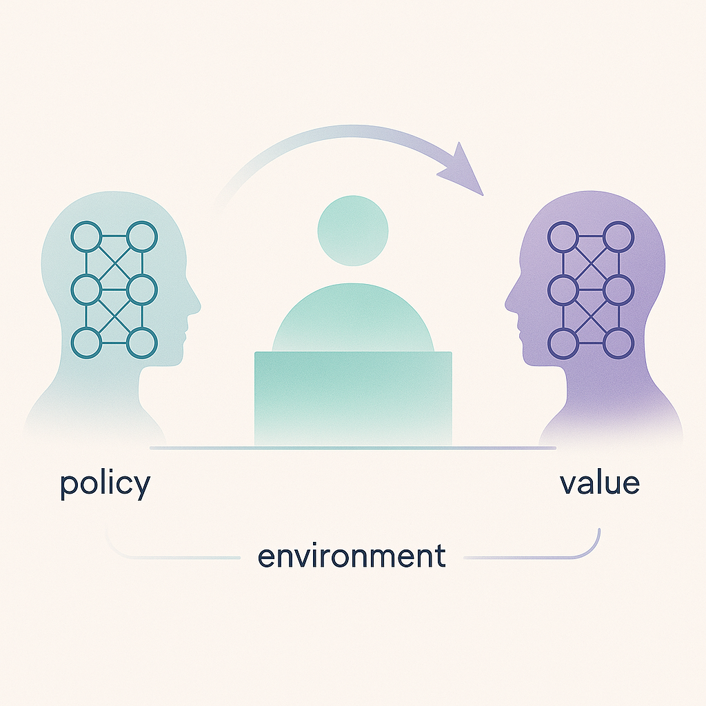
REINFORCE's variance problem is elegantly solved by a second estimator: the critic. This article motivates the baseline from first principles, derives the advantage function, shows the actor ↔ critic ↔ environment data flow as a Mermaid diagram and implements a runnable tabular actor-critic on the GridWorld mini world.
1. The Problem: REINFORCE Gradients Jitter
Article 02 ended with an open bill: REINFORCE is unbiased but high-variance. Concretely:
- A single episode with a random reward of +10 strongly shifts all gradients of that episode.
- Another episode with reward −5 shifts them just as strongly in the other direction.
- On average the direction is correct – but sample averaging needs thousands of episodes.
The central question: Can we subtract a reference value from the raw return $G_t$ to remove the "spread around the expectation" without distorting the direction?
2. The Baseline Trick: Mathematically Unbiased
We subtract a state-dependent baseline $b(s)$ from the return:
$$\nabla_\theta J(\theta) = \mathbb{E}\left[\nabla_\theta \log \pi_\theta(a \mid s) \cdot (G_t - b(s))\right]$$
The expectation does not change, because
$$\mathbb{E}{a \sim \pi}[\nabla\theta \log \pi(a \mid s) \cdot b(s)] = b(s) \cdot \nabla_\theta \underbrace{\sum_a \pi(a \mid s)}_{= 1} = 0.$$
The baseline can be anything as long as it does not depend on the action. The optimal baseline (in the sense of minimum variance) is the expected return from $s$ – exactly what we defined as the state value $V^\pi(s)$ in article 01.
3. From Baseline Trick to Advantage
Setting $b(s) = V^\pi(s)$ defines the advantage:
$$A^\pi(s, a) = Q^\pi(s, a) - V^\pi(s) \approx G_t - V^\pi(s)$$
In words: how much better was it to take action $a$ in $s$ than to follow the average action under $\pi$? Positive advantage → reinforce the action. Negative advantage → suppress the action. The learning logic gets drastically cleaner.
Quick check: What is the baseline $V(s)$ used for in policy gradients?
4. Actor-Critic: The Natural Architecture
If the baseline is to be learned, we need a second estimator – the critic $V_\phi(s)$. Two networks (or two heads on a shared backbone) are trained in parallel:
- Actor $\pi_\theta(a \mid s)$ – the policy. Updated by policy gradient with the advantage as weight.
- Critic $V_\phi(s)$ – the value estimator. Updated by TD loss against $r + \gamma V_\phi(s')$.
The critic watches what happens and estimates how "good" a state is on average. The actor uses that estimate as a reference to evaluate its own decisions. The two train each other up – similar to a chess player with a coach who does not move themselves but grades every move.
Quick check: What role does the critic play in actor-critic?
5. TD Bootstrapping: Shorter Returns, Lower Variance
A second lever for variance reduction besides the baseline is bootstrapping. Instead of summing the return $G_t$ over a whole episode we replace the tail with the critic:
| Estimator | Formula | Bias | Variance |
|---|---|---|---|
| Monte-Carlo (REINFORCE) | $G_t = \sum_{k=0}^{T-t} \gamma^k r_{t+k}$ | 0 | high |
| TD(0) | $\hat{G}t = r_t + \gamma V\phi(s_{t+1})$ | high | low |
| n-step | $r_t + \gamma r_{t+1} + \dots + \gamma^n V_\phi(s_{t+n})$ | medium | medium |
| GAE($\lambda$) | weighted mix of all n-step estimators | tunable | tunable |
Generalized Advantage Estimation (GAE) is the standard today. It defines:
$$\hat{A}t^{\text{GAE}(\lambda)} = \sum{l=0}^{\infty} (\gamma \lambda)^l \delta_{t+l}, \quad \delta_t = r_t + \gamma V_\phi(s_{t+1}) - V_\phi(s_t)$$
$\lambda = 0$ gives pure TD(0), $\lambda = 1$ Monte-Carlo. In practice $\lambda \in [0.9, 0.97]$ is common – PPO uses GAE directly.
6. Runnable: Tabular Actor-Critic on GridWorld
import numpy as np

rng = np.random.default_rng(0)
LENGTH = 7
GAMMA = 0.95
LR_A, LR_C = 0.1, 0.1
EPISODES = 2000

theta = np.zeros((LENGTH, 2))     # Actor logits per state
V     = np.zeros(LENGTH)           # Critic table

def softmax(x):
    z = x - x.max(); e = np.exp(z); return e / e.sum()

def policy_probs(s): return softmax(theta[s])

def step(s, a):
    s_next = max(0, min(LENGTH - 1, s + (1 if a == 1 else -1)))
    done = s_next in (0, LENGTH - 1)
    if done:
        r = 1.0 if s_next == LENGTH - 1 else -1.0
    else:
        r = 0.0
    return s_next, r, done

ep_returns = []
for ep in range(EPISODES):
    s = LENGTH // 2
    total = 0.0
    for _ in range(50):
        probs = policy_probs(s)
        a = int(rng.choice(2, p=probs))
        s_next, r, done = step(s, a)
        total += r

        # TD advantage instead of Monte-Carlo return.
        td_target = r + (0.0 if done else GAMMA * V[s_next])
        advantage = td_target - V[s]

        # Critic update (TD learning).
        V[s] += LR_C * advantage

        # Actor update (policy gradient with advantage as weight).
        grad_log = -probs.copy(); grad_log[a] += 1.0
        theta[s] += LR_A * grad_log * advantage

        s = s_next
        if done:
            break
    ep_returns.append(total)

print(f"Mean return (first 200) : {np.mean(ep_returns[:200]):+.3f}")
print(f"Mean return (last  200) : {np.mean(ep_returns[-200:]):+.3f}")
print("Learned V(s):")
for s in range(LENGTH):
    print(f"  s={s}: V={V[s]:+.2f}  P(right)={policy_probs(s)[1]:.2f}")
Compared to pure REINFORCE (article 02), this actor-critic converges noticeably faster and more stably – the critic averages away most of the noise. The learned $V$-values show a clear ramp from left (negative) to right (positive).
Quick check: Why does actor-critic converge faster than REINFORCE?
7. Bias-Variance Trade-off: The Real Game
Switching from Monte-Carlo to TD introduces bias – $V_\phi$ is wrong at the start, and that poisons the advantage. In exchange the variance drops dramatically. This trade-off is the core of almost every modern improvement:
- A2C/A3C – synchronous/asynchronous actor-critic with n-step.
- GAE – interpolation between MC and TD via $\lambda$.
- TRPO/PPO – trust region on top (see article 04).
- SAC – critic as $Q$-function instead of state value, off-policy with replay (see article 05).
"Reinforcement learning is, fundamentally, the management of bias and variance." – the practical RL engineer's job.
8. Shared vs. Separate Networks
A recurring design question: should actor and critic share weights?
| Variant | Pro | Con |
|---|---|---|
| Shared backbone | More efficient, shared representation | Competing loss signals, tricky weighting |
| Separate networks | Clean separation, independent tuning | More parameters, more memory |
PPO usually uses shared (with two heads), SAC almost always separate networks. On small state spaces the choice barely matters – on large vision inputs shared is worth it because CNN features help both.
9. Wrap-up Quiz
Which statement about actor-critic is correct?
What does the advantage $A(s, a)$ describe?
What is the effect of a too-small $\lambda$ in GAE?
What does 'on-policy' mean in the context of classical actor-critic methods?
What advantage comes from a shared backbone for actor and critic?
10. Further Reading
- Next article: Proximal Policy Optimization (PPO) (article 04 of this series).
- Cross reference: self-learning-agents/02-rl-fuer-code-agenten.
- Knowledge base:
masteringpytorch-secondedition.md– chapter on actor-critic.
Sources
- Sutton & Barto – Reinforcement Learning: An Introduction, 2nd ed., ch. 13 (Policy Gradient Methods).
- Schulman, J. et al. (2015) – High-Dimensional Continuous Control Using Generalized Advantage Estimation.
- Mnih, V. et al. (2016) – Asynchronous Methods for Deep Reinforcement Learning (A3C paper).